%pylab inline
import scipy.signal as dsp
Populating the interactive namespace from numpy and matplotlib
Uncertainty propagation for IIR filters
from PyDynamic.misc.testsignals import rect
from PyDynamic.uncertainty.propagate_filter import IIRuncFilter
from PyDynamic.uncertainty.propagate_MonteCarlo import SMC
from PyDynamic.misc.tools import make_semiposdef
Digital filters with infinite impulse response (IIR) are a common tool in signal processing. Consider the measurand to be the output signal of an IIR filter with z-domain transfer function
The measurement model is thus given by
As input quantities to the model the input signal values \(x[k]\) and the IIR filter coefficients \((b_0,\ldots,a_{N_a})\) are considered.
Linearisation-based uncertainty propagation
Scientific publication
A. Link and C. Elster,
“Uncertainty evaluation for IIR filtering using a
state-space approach,”
Meas. Sci. Technol., vol. 20, no. 5, 2009.
The linearisation method for the propagation of uncertainties through the IIR model is based on a state-space model representation of the IIR filter equation
where
The linearization-based uncertainty propagation method for IIR filters provides
- propagation schemes for white noise and colored noise in the filter input signal
- incorporation of uncertainties in the IIR filter coefficients
- online evaluation of the point-wise uncertainties associated with the IIR filter output
Implementation in PyDynamic
y,Uy = IIRuncFilter(x,noise,b,a,Uab)
with
xthe filter input signal sequencynoisethe standard deviation of the measurement noise in xb,athe IIR filter coefficientUabthe covariance matrix associated with \((a_1,\ldots,b_{N_b})\)
Remark
Implementation for more general noise processes than white noise is considered for one of the next revisions.
Example
# parameters of simulated measurement
Fs = 100e3
Ts = 1.0/Fs
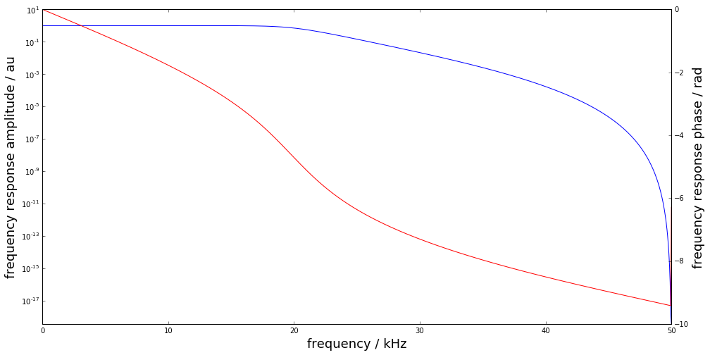
# nominal system parameter
fcut = 20e3
L = 6
b,a = dsp.butter(L,2*fcut/Fs,btype='lowpass')
f = linspace(0,Fs/2,1000)
figure(figsize=(16,8))
semilogy(f*1e-3, abs(dsp.freqz(b,a,2*np.pi*f/Fs)[1]))
ylim(0,10);
xlabel("frequency / kHz",fontsize=18); ylabel("frequency response amplitude / au",fontsize=18)
ax2 = gca().twinx()
ax2.plot(f*1e-3, unwrap(angle(dsp.freqz(b,a,2*np.pi*f/Fs)[1])),color="r")
ax2.set_ylabel("frequency response phase / rad",fontsize=18);
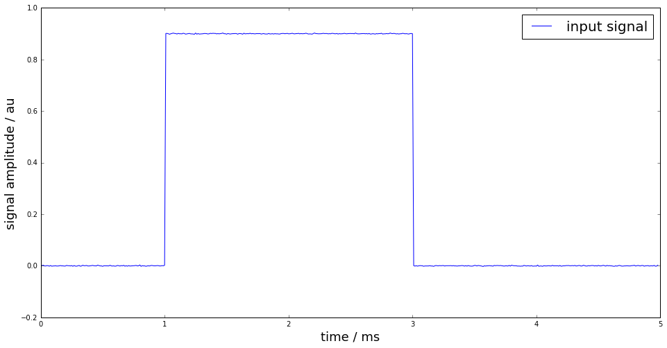
time = np.arange(0,499*Ts,Ts)
t0 = 100*Ts; t1 = 300*Ts
height = 0.9
noise = 1e-3
x = rect(time,t0,t1,height,noise=noise)
figure(figsize=(16,8))
plot(time*1e3, x, label="input signal")
legend(fontsize=20)
xlabel('time / ms',fontsize=18)
ylabel('signal amplitude / au',fontsize=18);
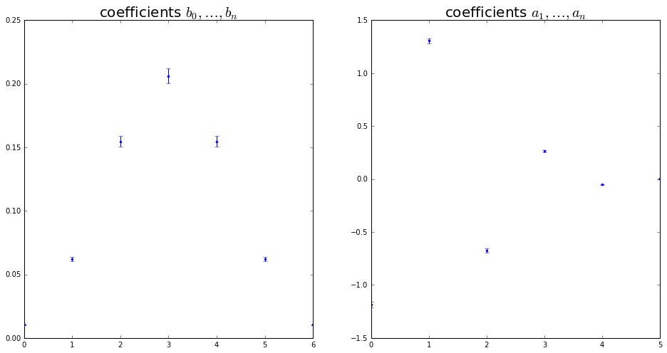
# uncertain knowledge: fcut between 19.8kHz and 20.2kHz
runs = 10000
FC = fcut + (2*np.random.rand(runs)-1)*0.2e3
AB = np.zeros((runs,len(b)+len(a)-1))

for k in range(runs):
    bb,aa = dsp.butter(L,2*FC[k]/Fs,btype='lowpass')
    AB[k,:] = np.hstack((aa[1:],bb))

Uab = make_semiposdef(np.cov(AB,rowvar=0))
Uncertain knowledge: low-pass cut-off frequency is between \(19.8\) and \(20.2\) kHz
figure(figsize=(16,8))
subplot(121)
errorbar(range(len(b)), b, sqrt(diag(Uab[L:,L:])),fmt=".")
title(r"coefficients $b_0,\ldots,b_n$",fontsize=20)
subplot(122)
errorbar(range(len(a)-1), a[1:], sqrt(diag(Uab[:L, :L])),fmt=".");
title(r"coefficients $a_1,\ldots,a_n$",fontsize=20);
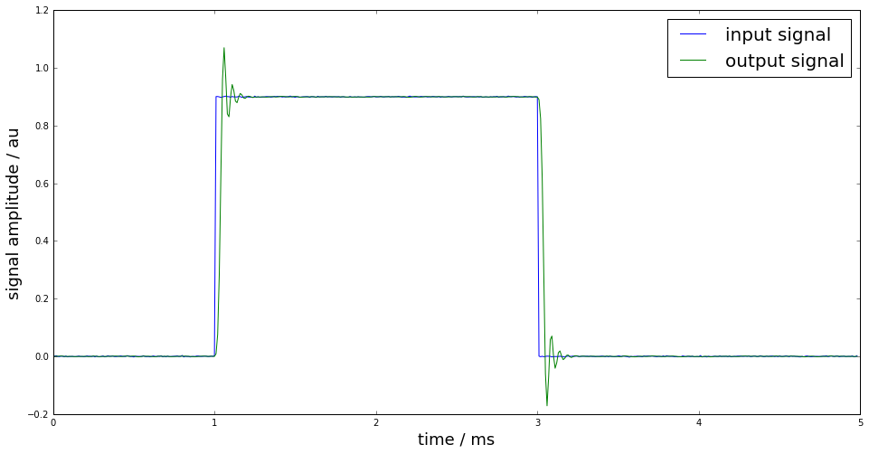
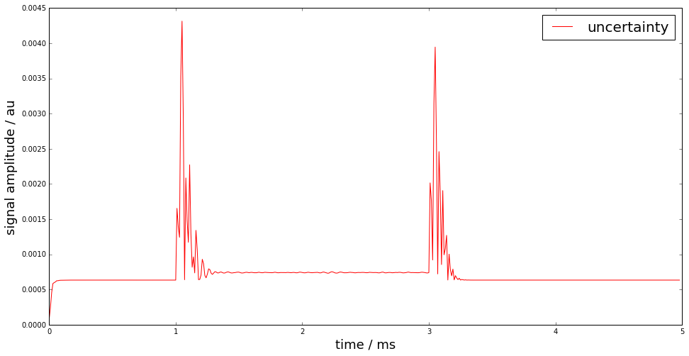
Estimate of the filter output signal and its associated uncertainty
y,Uy = IIRuncFilter(x,noise,b,a,Uab)

figure(figsize=(16,8))
plot(time*1e3, x, label="input signal")
plot(time*1e3, y, label="output signal")
legend(fontsize=20)
xlabel('time / ms',fontsize=18)
ylabel('signal amplitude / au',fontsize=18);
figure(figsize=(16,8))
plot(time*1e3, Uy, "r", label="uncertainty")
legend(fontsize=20)
xlabel('time / ms',fontsize=18)
ylabel('signal amplitude / au',fontsize=18);
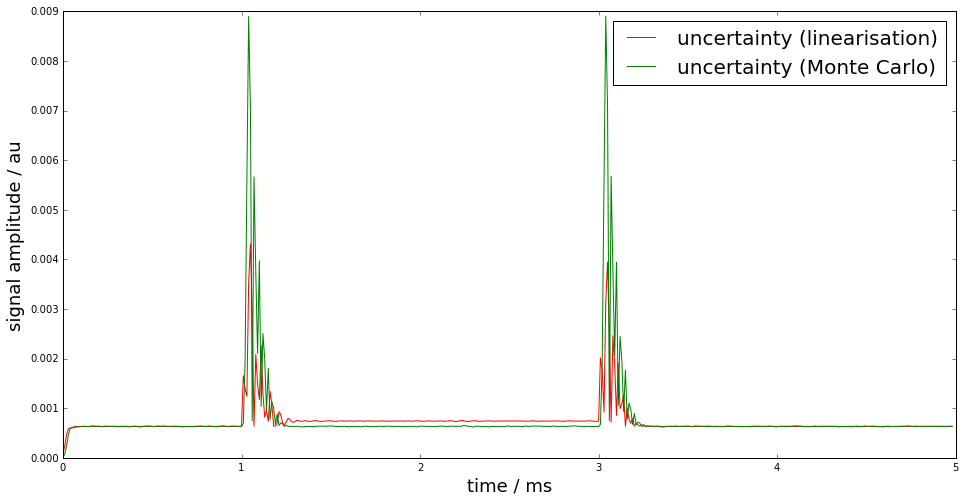
Monte-Carlo method for uncertainty propagation
The linearisation-based uncertainty propagation can become unreliable due to the linearisation errors. Therefore, a Monte-Carlo method for digital filters with uncertain coefficients has been proposed in
S. Eichstädt, A. Link, P. Harris, and C. Elster,
“Efficient implementation of a Monte Carlo method
for uncertainty evaluation in dynamic measurements,”
Metrologia, vol. 49, no. 3, 2012.
The proposed Monte-Carlo method provides - a memory-efficient implementation of the GUM Monte-Carlo method - online calculation of point-wise uncertainties, estimates and coverage intervals by taking advantage of the sequential character of the filter equation
yMC,UyMC = SMC(x,noise,b,a,Uab,runs=10000)

figure(figsize=(16,8))
plot(time*1e3, Uy, "r", label="uncertainty (linearisation)")
plot(time*1e3, UyMC, "g", label="uncertainty (Monte Carlo)")
legend(fontsize=20)
xlabel('time / ms',fontsize=18)
ylabel('signal amplitude / au',fontsize=18);
SMC progress: 0% 10% 20% 30% 40% 50% 60% 70% 80% 90% 100%